An overview of computational methods for molecular modeling

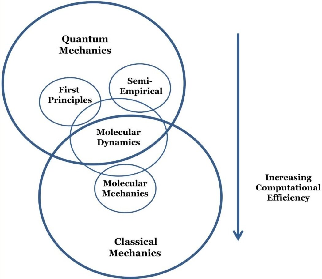
Bazargan, G., & Sohlberg, K. (2018). Advances in modelling switchable mechanically interlocked molecular architectures. International Reviews in Physical Chemistry, 37(1), 1-82.

Computational methods for molecular modeling can be separated into two categories: those that are based on quantum mechanics (QM) and those that are based on classical mechanics. When choosing a computational method, one should consider the type of information desired and the speed of the calculations. Here I briefly describe these methods.

Molecular mechanics (MM) methods involve using an empirical potential energy function called a ‘force field’ to describe the energy of the system as a function of its configuration. The function is constructed by empirically fitting a guessed equation so that it produces experimentally-confirmed results for a defined set of molecules and does not need to have any physical or chemical basis. Properties are extracted from the empirical potential energy function using numerical methods. Electronic properties of the system are treated only implicitly by the empirical parameters in the force field. While MM methods are useful for rapid structural optimizations, they cannot provide any electronic structure information.

Molecular dynamics (MD) simulations time propagate the dynamical behavior of a system and can use MM or QM potential energy functions. Given an initial state of the system, Newton’s equations of motion are solved numerically so that the time development of the state of the system is followed. MD methods are useful for conformational searching or determining statistically-averaged quantities. One limitation of MD is that the simulation time is finite and very long simulations or a series of shorter simulations may be needed to ensure sufficient sampling.

First principles methods are based on QM. This category includes both wavefunction-based and density-functional methods. These methods solve the time-independent Schrödinger equation by employing only mathematical approximations. All electrons in the system are treated, and electronic structure information is obtained. In principle, they are the most accurate of all computational methods. In practice, however, they are impractical for large systems due to the fact they become prohibitively computationally expensive at a much smaller system size than most other techniques. Examples of wavefunction methods are: Hartree–Fock, Møller–Plesset perturbation theory, and coupled cluster techniques. Unlike wavefunction methods, density functional theory (DFT) methods extract the energy and other system properties from the electronic density instead of the electronic wavefunction.

Semi-empirical methods are based on both QM and empirical parameters. These methods only treat valence electrons explicitly and treat inner shell electrons implicitly. The time-independent Schrödinger equation is solved but integrals that are difficult to solve analytically are approximated by empirical parameters. SE methods provide electronic structure information at a lower computational cost than first principles methods.